Diffusion Language Models: Some Nice Visualizations
Some (hopefully) Nice visualizations for understanding diffusion LMs
Continuous Diffusion Language Models: Some Nice Visualizations
Patrick Pynadath, Ruqi Zhang
Diffusion large language models (dLLMs) are starting to show benefits over auto-regressive counterparts, particularly since the introduction of Mercury 2, which is described as “the fastest reasoning LLM”. By matching / outperforming AR counterparts while providing significant throughput advantages, the advantages of dLLMs are become more widely known.
The goal of this blog is to provide some nice visualizations and background on continuous diffusion LLMs for those who may be interested. As my focus is primarily on continuous dLLMs, I focus on visualizing and discussing some recent discoveries within this field. I hope that this is helpful for those starting to learn about this field, as it was certaintly difficult for me to visualize adding Gaussian noise to language.
Contents
While not the focus of this blog, it may be helpful to visualize discrete denoising approaches to contextualize how continuous denoising differs.
Masked Diffusion
Masked diffusion involves replacing tokens in a sequence with a mask token as the primary means of corruption [1]. The noising process interpolates between a fully masked state, where every token is replaced with a mask, and the original clean sequence. This approach is particularly popular as training just requires predicting the masked tokens across various levels of corruption [2] [3].
Masked diffusion models have nice connections to other approaches for discrete generative modeling. First, the training objective commonly used for these models can be thought of as a reweighted masked language modeling objective (MLM) from BERT [4] [2] [3]. While there have been previous attempts at using BERT as a generative model [5], the success of masked dLLMs involved training the bidirectional encoders across a range of discrete corruption as opposed to a single fixed corruption rate. Furthermore, the trajectories produced by masked dLLMs are mathematically equivalent to any-order autoregression, where tokens are predicted one at a time, but in any arbitrary order beyond just left to right [6].
Uniform Diffusion
Uniform corruption involves interpolating between the clean sentence and a sequence sampled from a uniform distribution across all tokens [7]. We include a visualization of this process below.
As visible, each position can change token identity multiple times within the same process. This differs from masked diffusion, which restricts a token from changing after it transitions from a masked state. This property of uniform diffusion is desirable, as it should enable the model to correct its own mistakes during generation [8].
Continuous Denoising
While discrete denoising has arguably seen the most success within the language modeling context, applying continuous denoising methods towards language modeling has remained an active field of research.
Here we visualize the decorruption of a noisy latent under a linear interpolation schedule. We use the words spreading out to visualize the continuous denoising process, and the “flipping” of the bold tokens to represent discrete decorruption, or when the continuous latent becomes closest to the correct token. We visualize this for a vocabulary of 50,257 words, which correspends to the number of unique tokens for GPT-2.
Discrete Corruption of Continuous States
Even when considering continuous denoising, it is possible to characterize the effect of Gaussian noise in terms of discrete corruption [8]. Recent work has demonstrated that Gaussian noise induces undesirable scaling with vocabulary size: with a sufficiently large vocabulary size, most of the discrete corruption becomes concentrated towards the end of the denoising process [9], [10]. In our recent work [10], we called this a temporal dissonance to reflect the misalignment between continuous and discrete corruption with large vocabularies. We visualize this below — with a vocabulary size of 50, discrete decorruption is relatively spread throughout the process. When we scale to 50,257, discrete decorruption becomes concentrated within a narrow band of the denoising process.
 Here we show the discrete corruption effect simulated for a vocabulary size of 5. The discrete decorruption is relatively spread out.
 Here we show the discrete corruption effect simulated for a vocabulary size of 50,257. The discrete decorruption is concentrated towards the end, with all positions being decorrupted at almost the same time.
Why Continuous Language Models need Discrete Structure
It may not be immediately clear why continuous language models should need to be concerned with discrete corruption. The short explanation is that discrete conditional dependencies need to be learned, whereas continuous conditional dependencies have an inherently smooth structure where nearby pixels share similar values.
Conditional Structure in Language
Consider the masked sentence below.
I live in [Mask] York City. The reader will probably recognize the mask token should be “New”. This is not due to “New” or “York” being semantically similar on their own, or being similar in terms of characters — it is because “York City” is usually preceded by “New” whenever the former appears in text. In other words, the conditional relation between “York City” and “New” is something observed through data — not through anything inherent to the words themselves.
Conditional Structure in Natural Images
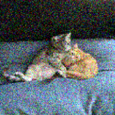
In contrast, take this noisy picture of two cats. While the image is blurry, it is clear what colors the pixels should be — the noisy pixels on the bottom should be blue, in the middle should be gray, and the top should be black. The reader could probably infer these despite never seeing these cats. This is because images are spatially smooth — nearby pixels tend to share similar values. Thus the sample itself has a correlational structure that is not dependent on previous data or information.
In summary, the conditional structure within language must be learned — even if a noisy position is right next a clean position, there is no way to tell what word the noisy position should be without some knowledge on what words belong together. Within images, it can be assumed that nearby pixels will tend to have similar values (except for high frequency features, like edges, etc).
In order for a model to learn what words go together, it seems necessary to train the model to condition on some words that retain their original identity and predict the remaining words. The amount of clean words the model can use to condition is determined by the discrete corruption level, which is why this quantity is being more carefully controlled within recent work [9] [10].
The same explanation may not apply to continuous denoising applied to latent representations. For such methods, the information for each token is spread throughout the entire representation being noised. However, such methods have typically found that while the denoising does not require discrete conditioning, the representation learning phase still does.
Noise Reparameterization
One way to avoid the problematic behavior of Gaussian noise with large vocabularies is to reparameterize the time for the denoising process to be linear with respect to discrete corruption [9]. By enabling pure continuous denoising to better capture discrete conditional dependencies, it becomes possible to adapt distillation techniques from continuous flow matching towards language modeling, which is a promising direction for even quicker few-step language generation [11] [9].
Hybrid Methods
Another way of avoiding the temporal dissonance is by simply decoupling discrete from continuous noise by using an addition discrete noising schedule. Decoupling the two forms of corruption enables independent control over each one, which allows for learning both discrete and continuous geometry simultaneously.
Fun Widget
Below is a small interactive widget that allows the user to move through the denoising processes for the methods discussed in this blog. Hopefully this provides a nice visual intuition as to how these methods denoise language — particularly the continuous approaches, as it wasn’t clear to me how to visualize continuous noise for language.